In 1881, Francis Y. Edgeworth came up with a way of representing, using the same axis, indifference curves and the corresponding contract curve in his book “Mathematical Psychics: an Essay on the Application of Mathematics to the Moral Sciences”. It was Vilfredo Pareto, in his book “Manual of Political Economy”, 1906, who developed Edgeworth’s ideas into a more understandable and simpler diagram, which today we call the Edgeworth box.
Edgeworth box a conceptual device for analyzing possible trading relationships between two individuals or countries, using indifference curves. It is constructed by taking the indifference map of one individual (B) for two goods (X and Y) and inverting it to face the indifference map of second individual (A) for the same two goods. Thus, Edgeworth box is a traditional visualization of the benefits potentially available from international trade.
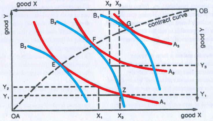
Individual A’s preferences are depicted the three indifference curves A1, A2 and corresponding to higher levels of satisfaction as we move outward from origin OA. Individual B’s preferences are depicted by the three indifference curves B2 and B3, corresponding to higher levels satisfaction as we move outward from origin OB. Both consumers’ preferences between the reflected in the slopes of their indifference curves, with the slope of a curve at any point reflecting the Marginal Rate of Substitution of X for Y. Only where individual A’s indifference curves are tangential to individual B’s indifference curves (points E, F and G) will A’s marginal rate of substitution of product X for product Y be the same as B’s marginal rate of substitution of X for Y, so that their relative valuations of the two products are the same. Starting from any other point, say Z, the two can gain by trading with one another.
At point Z, individual A has a lot of product X and little of product Y; consequently, he values product Y more highly than product X, being prepared to give up a lot of product X (X1 X3) to gain just a little of product Y (Y1 Y2). This is why his indifference curve A1 is relatively flat at point Z. On the other hand, at point Z individual B has a lot of product Y and little product X; consequently, he values product X more highly than product Y, being prepared to give up a lot of product Y (Y1 Y3) to gain just a little of product X (X2 X3). This is why his indifference curve B2 is relatively steep at point Z.
These two sets of relative valuations of product X and product Y offer the promise of mutually beneficial exchange. If individual A offers some of his plentiful and low €valued product X in exchange for extra units of scarce and high €valued product Y, he can gain from trade. Similarly, if individual B offers some of his plentiful and low €valued product Y in exchange for extra units of scarce and high €valued product X, he can also gain from trade. The two will continue to exchange product X in return for product Y (individual A) and product Y in return product X (individual B), until they reach point, such as E or F, where the indifference curves have the same slope, so that their marginal rates of substitution of the two products are the same.
The curve which is drawn from origin to origin is called a contract curve and it joins together all tangency points of the two consumers’ indifference curves. It is called the contract curve since voluntary negotiations which does not leave out any possibilities for mutually advantage trades (so called “efficient bargaining”) could be predicted to end up somewhere on this curve, the exact point depending on the starting point, i.e., the position of the endowment point.
The contract curve or offer curve in figure traces out the path of all the points, such E, F and G, where the indifference curves tangential, and individual A and B start with any combination of products X and other than ones lying along the contract curve, then they have an incentive to redistribute products X and Y between themselves through exchange. Where they come to lie along the contract curve will depend upon their relative bargaining strength and skills. If individual A is the stronger, they may end up at a point like far from A’s origin, OA, and putting individual A on a high indifference curve, A3 while individual B ends upon a low indifference curve B1 near his origin, OB. On the other hand, if individual B is the stronger, they may end up at a point like E, far from B’s origin, OB, and putting individual B on a high indifference curve, B3 while individual A ends up on a low indifference curve,A1, near his origin, OA.
What points are efficient? The economic notion of efficiency is that an allocation is efficient if it is impossible to make one individual better off without harming the other individual; that is, the only way to improve A’s utility is to harm B, and vice versa. Otherwise, if the consumption is inefficient, there is a rearrangement that makes both parties better off, and the parties should prefer such a point. Now, there is no sense of fairness embedded in the notion, and there is an efficient point in which one person gets everything and the other gets nothing. That might be very unfair, but it could still be the case that improving B must necessarily harm A. The allocation is efficient if there is no waste or slack in the system, even if it is wildly unfair. To distinguish this economic notion, it is sometimes called Pareto efficiency. We can find the Pareto-efficient points by fixing Individual A’s utility and then asking what point, on the indifference isoquant of Individual A, maximizes Individual B’s utility. At that point, any increase in Individual B’s utility must come at the expense of Individual A, and vice versa; that is, the point is Pareto efficient.