The risk or variation in return of a security is caused by two types of factors. The first type of factors will affect the return of almost all securities in the market. Examples of such sources of risks are changes in the interest rates and inflation of the economy, movement of stock market index and exchange rate movement. The risk caused by such factors is known as systematic risk. Apart from systematic risk, the variation in return of a security is also caused by some other factors which are specific to a security, like a strike in a company or the caliber of the management of a company. The risk caused by such factors is known as unsystematic or specific risk. The unsystematic risk of a security can be diversified away by combining different securities into a portfolio. But systematic risk cannot be diversified away by the construction of a portfolio. So the real risk of a security is the systematic risk as the investors can diversify the unsystematic risk by the construction of a portfolio. The systematic risk of a security is measured by a statistic known as beta. The beta of security measures the sensitivity of a security’s return to changes in the return of the market portfolio or stock market index. Introduced and developed in the early 1960’s, the Capital Asset Pricing Model (CAPM) demonstrates the link between the risk and return of an asset, in a reasonable equilibrium market. The aim of the CAPM formula is to assess whether a stock is valued fairly when considering risk and time value of money, compared to its expected return.
Capital Asset Pricing Model (CAPM)
In the 1950s, Harry Markowitz introduced the Modern Portfolio Theory (MPT), being among one of the first to discuss the relationship between risk and the rate of return. This theory argues that the characteristics of an investment’s risk and return shouldn’t be considered solely but should recognize the broad impact the investment has on the portfolio’s risk and return. The MPT assumes that investors are all risk averse, which means they will opt for the least risky asset when investing, given its level of return. This suggests that an investor will engage in more risky investments, with the expectation of a higher return.
Originally introduced by William Sharpe (1964), Jack Treynor (1962), John Lintner (1965) and Jan Mossin (1966), the Capital Asset Pricing Model (CAPM) builds upon concepts from the Modern Portfolio Theory, yet based on the concept that the price of an asset should not always be dependent on its risk. CAPM is a theoretical representation of the behavior of financial markets, can be employed in estimating a company’s cost of equity capital. The MPT demonstrates how rational investors should build a profitable portfolio regarding their risk-return preferences. Whereas, the CAPM includes a relationship, expanding on how assets should be priced in the capital market. CAPM holds that the expected return of a security or a portfolio equals the rate on a risk-free security plus a risk premium. If this expected return does not meet or beat a theoretical required return, the investment should not be undertaken.
The Capital Asset Pricing Model (CAPM) is a general equilibrium market model developed to analyze the relationship between risk and required rates of return on assets when they are held in well-diversified portfolios. The Capital Asset Pricing Model (CAPM) provides a linear relationship between the required rate of return (Ri) of a security and its Systematic or undiversifiable risk as measured by the security’s beta. The systematic risk of a security, which is measured by the beta coefficient of the security, is the market risk that cannot be eliminated through diversification.
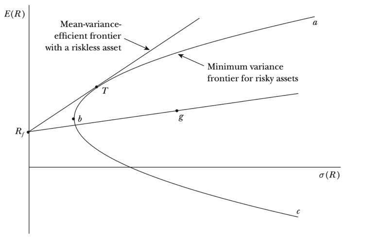
The graph below illustrates portfolio opportunities and explains the story of CAPM. The axis which runs horizontally across indicates portfolio risk which is measured by the standard deviation of portfolio return. The axis that’s vertical, illustrates the expected return. The abc curve (known as the minimum variance frontier) demonstrates the combination of expected return and the risk of assets which minimize return.
The CAPM requires an extensive set of assumptions:
- All investors are single-period expected utility of terminal wealth maximizers, who choose among alternative portfolios on the basis of each portfolio’s expected return and standard deviation.
- All investors can borrow or lend an unlimited amount at a given risk-free rate of interest.
- Investors have homogeneous expectations (that is, investors have identical estimates of the expected values, variances, and covariances of returns among all assets).
- All assets are perfectly divisible and perfectly marketable at the going price, and there are no transaction costs.
- There are no taxes.
- All investors are price takers (that is, all investors assume that their own buying and selling activity will not affect stock prices).
- The quantities of all assets are given and fixed.
According to the Capital Asset Pricing Model approach, the required return on a security is given by the equation:
Ri = Rf + βi ( Rm — Rf )
Where,
- Ri = Required rate of return on security i or cost of equity.
- Rf = Risk-free rate of return.
- βi = Beta of security i.
- Rm = Rate of return on the market portfolio.
Security Market Line (SML) Analysis
The graphical plot of the relationship between the required rate of return (ke) and the non-diversifiable risk (beta) of security is known as Security Market Line (SML).

The CAPM model uses the Security Market Line (SML), which is a tradeoff between expected return and security’s risk (beta risk) relative to the market portfolio. Under equilibrium conditions, any individual securities expected return and beta should lie on the SML. Since all securities are expected to plot along the SML, the line provides a direct way of determining the expected (required) return of a security once the beta of the security is known.
It is useful to compare the security market line (SML) to the capital market line (CML). The CML graphs the risk premiums of efficient portfolios (i.e., portfolios composed of the market and the risk-free asset) as a function of portfolio standard deviation. This is appropriate because standard deviation is a valid measure of risk for efficiently diversified portfolios that are candidates for an investor’s overall portfolio. The SML, in contrast, graphs individual asset risk premiums as a function of asset risk. The relevant measure of risk for individual assets held as parts of well-diversified portfolios is not the asset’s standard deviation or variance; it is, instead, the contribution of the asset to the portfolio variance, which we measure by the asset’s beta. The SML is valid both for efficient portfolios and individual assets.
The security market line provides a benchmark for the evaluation of investment performance. Given the risk of an investment, as measured by its beta, the SML provides the re quired rate of return necessary to compensate investors for both risk as well as the time value of money. Because the SML is the graphic representation of the expected return-beta relationship, ‘fairly priced’ assets plot exactly on the SML; that is, their expected returns are commensurate with their risk. Given the assumptions we made at the start of this chapter, all securities must lie on the SML in market equilibrium.
If a stock is perceived to be a good buy, or under-priced, it will provide an expected return in excess of the fair return stipulated by the SML. Under-priced stocks therefore plot above the SML: given their betas, their expected returns are greater than dictated by the CAPM. Overpriced stocks plot below the SML.
Empirical Tests for Capital Asset Pricing Model (CAPM)
Since the Capital Asset Pricing Model (CAPM) was developed on the basis of a set of unrealistic assumptions, empirical tests should be used to verify the CAPM.
The first test looks for stability in historical betas. If betas have been stable in the past for a particular stock, then its historical beta would probably be a good proxy for its ex-ante, or expected beta. Empirical work concludes that the betas of individual securities are not good estimators of their future risk, but that betas of portfolios of ten or more randomly selected stocks are reasonably stable, hence that past portfolio betas are good estimators of future portfolio volatility.
The second type of test is based on the slope of the SML. As we have seen, the CAPM states that a linear relationship exists between a security’s required rate of return and its beta. Further, when the SML is graphed, the vertical axis intercept should be RF, and the required rate of return for a stock (or portfolio) with beta = 1.0 should be Rm, the required rate of return on the market. Various researchers have attempted to test the validity of the CAPM model by calculating betas and realized rates of return, plotting these values in graphs, and then observing whether or not (1) the intercept is equal to RF, (2) the regression line is linear, and (3) the SML passes through the point b = 1.0, Rm. Evidence shows a more-or-less linear relationship between realized returns and market risk, but the slope is less than predicted. Tests that attempt to assess the relative importance of market and company-specific risk do not yield definitive results, so the irrelevance of diversifiable risk specified in the CAPM model can be questioned.
In general, evidence seems to support the CAPM model when it is applied to portfolios, but the evidence is less convincing when the CAPM is applied to individual stocks.
Nevertheless, the CAPM provides a rational way to think about risk and return as long as one recognizes the limitations of the CAPM when using it in practice.
Recent Developments of the Capital Asset Pricing Model
Since being introduced, many researchers have decided to extend and develop the standard Capital Asset Pricing Model since the 1960s. Asset pricing models have evolved considerably with the aim of improving their realism.
Three-Factor Model
One critical assumption in CAPM is the risk premium estimation, the residual between the market return and the risk-free interest rate. The Three-Factor Model was developed and proposed by Fama and French in response to accumulating empirical evidence that the CAPM performed poorly in explaining realized returns. When developing the standard CAPM, Fama and French added two factors with the aim of better explaining the returns of the portfolio, including market capitalization and book-to-market value. In 1995, they identified a covariance between the company’s book-to-market ratio and size, with the aim of measuring the return of the stock. After testing the Three-Factor Model empirically, it was confirmed that this model had higher explanatory power than the one-factor CAPM. This means that the main advantage of this model is that it includes the size and value of the firm, and the market risk factor used in the CAPM.
Five-Factor Model
After developing the three-factor model, Fama and French went on to further expand on this theory, introducing the Five-Factor model. This model was directed at not only taking into consideration the size and value of the firm, and the market risk factor – but it also considers the profitability of the stocks and the investment patterns in average stock returns. The empirical tests of the five-factor model aim to explain average returns on portfolios formed to produce large spreads in size, profitability, and investment. With the addition of profitability and investment factors, the value of the previous three-factor model becomes redundant.
Arbitrage Pricing Theory (APT)
Like CAPM, this theory gives investors an estimated required rate of return on portfolios that are of risk. The Arbitrage Pricing Theory aims to reduce the limitations of the one-factor CAPM, with the understanding that different stocks will have alternative sensitivities to different market factors. The APT bases its assumption on the fact that an asset is dependent on numerous macroeconomic factors, i.e. inflation, exchange rates, market indices, changes in interest rates, and market sentiments, to name a few. Simply, not all assets or stocks can be expected to react to a specific and same parameter all the time, thus the requirement to consider the multifactor and sensitivities.
Zero-Beta CAPM
Developed by Black in 1972, the Zero-Beta CAPM showed that the results from CAPM do not require a risk-free asset that has returns constantly in every state of nature. A zero-beta portfolio is one that is built without systematic risk. The zero-beta CAPM implies that beta is still the correct measure of systematic risk and that the model still has a linear specification. This means that the value of the portfolio doesn’t fluctuate with market movements. Without systematic risk in a zero-beta portfolio, the return is the same as the risk-free rate. Thus, the return on a portfolio with zero-beta is going to below, and without the volatility of the market exposed, it does not allow the portfolio to benefit from potential upswings in value of the overall market.
Inter-Temporal CAPM
ICAPM focuses on relaxing the single time period assumption from the standard CAPM. It is said that investors who use ICAPM are only concerned with the end-of-period payoff, as well as the chance to consume or invest this payoff., whereas investors of the standard CAPM would be interested in the wealth of their assets at the end of the current period. With the Inter-temporal CAPM, there is the assumption of a perfect market; no costs or taxes, all assets have limited liability, investors believe their decision has no impact on the market price and the market is always in equilibrium, etc. It’s evident that the ICAPM extends the CAPM to a more dynamic environment, where the results almost mirror that of the APT. The difference between ICAPM and APT, however, is that the ICAPM has the ability to determine risks from characteristics of the assets.
Downside CAPM (Downside BETA)
Downside BETA or Downside-CAPM is another extension from the CAPM. This concept dates back to Beta is used within the standard CAPM as a way of calculating the expected return of an asset. Downside beta is a way to measure the downside risk of an asset, the risk associated with loss. Investors may try and consider constructing their portfolios by minimizing the downside beta. The reason for this is to ensure they can maintain the value in times of market decline.
Revised CAPM
This model is a further development of the standard Capital Asset Pricing Model, which includes financial, operational, and economic leverages. In order to achieve a more accurate prediction of return, it focuses on systematic and unsystematic risk, including historical and estimating data completely. When testing this model, they compared R-CAPM with the traditional CAPM, Downside CAPM, and the Adjusted-CAPM, and found that there was a meaningful difference between the measures of expected return for R-CAPM and the alternative CAPMs.
Consumption CAPM (Co-CAPM)
The Consumption CAPM is an additional extension of the standard CAPM. Co-CAPM quantity market risk is measured by the movement of the premium with consumption growth. Thus, the Co-CAPM explains how much the entire stock market changes related to consumption growth. This model is argued to be the best theoretical model, however, the basic link between consumption and stock returns assumed by the Co-CAPM cannot hold. The Co-CAPM is used more from an academic perspective as it covers many forms of wealth, beyond stock market wealth, providing an understanding of variation in returns over a number of periods.
Reward CAPM (Reward-BETA)
It was stated by Graham Bornholt in 2006, that investors require a better methodology in order to estimate the expected returns within the stock market. With this in mind, he developed the Reward-BETA CAPM. This model is based on assumptions that are consistent with the Arbitrage Theory; dividing returns of stocks into two parts: expected and unexpected stock returns.